

Microsoft office is probably the first thing you learn while taking a computer course. It is one of the basic steps while learning about computer operations. In Microsoft office, we learn how to operate Word, Excel, PowerPoint, etc. Yet we know nothing about its operations. This is because we are taught only those things which are absolutely necessary.
It is only when you start working, you realise that in Microsoft Office, there are so much you don’t know about and there are so many new things to learn everyday. Let us take the most common used function in excel, the Vlookup function.
What is Vlookup?
The V in the Vlookup stands for vertical. So you can match up the value of a cell from a (vertical) row and look up its value of any desired column matching the searched cell, from another sheet/row/different excel sheet.
How Does it work?
There are two sheets; Sheet1 & Sheet2. The Cell values of Row 1 is same, but there are some Rows added in Sheet2 which are not there in Sheet1. So what to do?
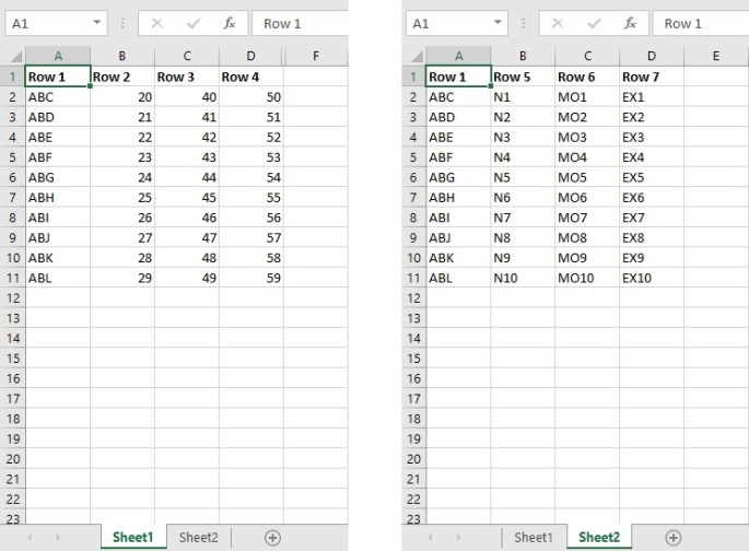
Now in this case the value of Row1 in Sheet1 matches with Row1 from sheet2. So you can copy and paste the rows 5,6 & 7 from one sheet to another. But that’s not what we are going to do now. Now we are going to use vlookup function to take the value of one cell to another.
Here’s the formula: =VLOOKUP(A2,Sheet2!A:B,2,0)

How does the formula works?
First, write the vlookup formula followed by ‘(“, after that, select the cell you want to find in another row. In the above picture, you can see, the value of cell A2 in Sheet1 is ‘ABC’. I wanted to find that in Sheet2.
After that, select the range of the table (here I have selected the rows A&B).
After that, select the vale of the column from which the data will be pulled from (here I have selected the second column).
Lastly, you have to define what type of search you want to do. Would you want the value to be exact match or approximate match. You can either write True / 1 or False / 0.
Now similarly, for other rows you can use the formula:
=VLOOKUP(A2,Sheet2!A:C,3,0)
=VLOOKUP(A2,Sheet2!A:D,4,0)
*Note: There are some restrictions in vlookup function. The searched value should contain in the first row of the lookup. The values will only be extracted from the column from right (Not Left).
Hope this blog helps you understand the vlookup function. Let me know in the comment if you want other information about vlookup.
